Use the sphere model described in the “Getting Started with CAPITOLE-RCS” example.
The file is sphere200mm.step
RCS of a sphere as a function of frequency
This document presents an RCS simulation of a sphere with CAPITOLE-RCS.
The model used is a simple sphere with a radius of 0.2 m.
The monostatic RCS calculation will be performed in one direction and for a frequency sweep from 10 MHz to 8 GHz.
File :
1.geometric model

2.simulation strategy
In this case, the frequency range is very wide, from 10 MHz to 8 GHz.
As CAPITOLE-RCS is based on a frequency domain method, it is not advisable to use a single mesh for the entire frequency sweep.
Instead, you should create several CAPITOLE-RCS projects for a sub-band of the frequency range, and use a mesh model adapted to that frequency range.
Remember that the mesh size must always be less than or equal to λ/10 at the highest frequency.
| File name | Frequency range | # Number of triangles | Mesh size | Solver | Calculation time | sphere100.h5 | 10-100 MHz | 1380 | λ/1026 - λ/102 | Full | 3s |
|---|---|---|---|---|---|
| sphere1000.h5 | 100-1000 MHz | 1380 | λ/102 - λ/10 | Full | 29s |
| sphere2000.h5 | 1000-2000 MHz | 5426 | λ/20 - λ/10 | MLACA | 1min42s |
| Sphere3000.h5 | 2000-3000 MHz | 12194 | λ/15 - λ/10 | MLACA | 4min22s |
| sphere4000.h5 | 3000-4000 MHz | 21664 | λ/13 - λ/10 | MLACA | 7min6s |
| sphere5000.h5 | 4000-5000 MHz | 33858 | λ/13 - λ/10 | MLACA | 11Min26s |
| sphere8000.h5 | 5000-8000 MHz | 136 264 | λ/16 - λ/10 | MLACA | 1h15min18s |
The MLACA solver is the most efficient, as it uses impedance matrix compression. But at low frequencies, the electrical mesh size becomes smaller and it is impossible to use the MLACA solver when the mesh size is less than λ/100, instead it is possible to use the Full solver.
All simulations were run on a DELL PowerEdge R920 server with 4 Intel Xeon E7-8857 v2 3.0 GHz 12-core CPUs, 512GB memory.
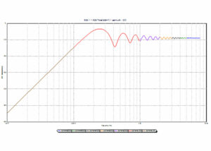
All project files can be opened with POSTPRO3D at the same time. A single graph can display all results.
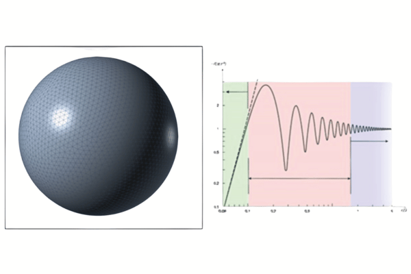
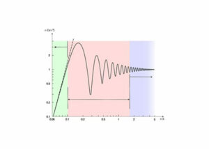
There are 3 regions of a sphere’s SCR. They can be seen on this graph.
The Rayleigh region, when λ>10 r
For a 0.2 m sphere, it extends to 150 MHz.
The creeping wave effect occurs when λ=2πr
This corresponds to a frequency of 239 MHz where there is a maximum of RCS.
The optical region begins when 2πr/λ>10
For a 0.2 m sphere, this corresponds to 2.39 GHz.
Above this frequency, the sphere’s SCR is independent of frequency and equal to:
σ= πr^2
For a 0.2 m sphere, σ = -9 dBm².
And between the Rayleigh region and the optical region is the Mie region.
Test CAPITOLE RCS
Explore the possibilities offered by CAPITOLE RCS today