Open the FreeCAD software.
(FreeCAD version 0.19 was used, but any version will do)
Click on“New” to create a new project
Select“Part“.
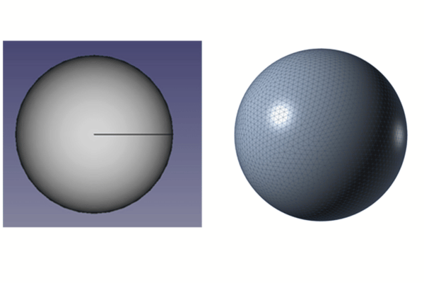

Click on the“sphere” button![]()
Select the“Sphere” object from the tree
Change the radius to ” 0.2 m “.


Select the “ STEP ” file type and select the sphere200mm.step file
In the project panel, set the frequency
Click on the ![]()
button Enter a single frequency of 2.5 Ghz

Create a source ![]()
Click on PlaneWave for this source
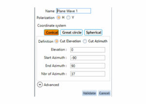

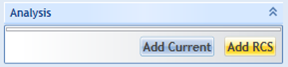
Create an RCS analysis :


In the Solver menu, click on“Run“.


Click on“Run“
The calculation starts.
The process uses 1.9 GB RAM memory
The calculation takes 36 s on a laptop with an Intel Core i7-7700HQ processor.
When the calculation is complete, click on“POSTPRO” in the“Tools” menu.

